
[mathjax]
为了带师弟做实验,简要总结一下在MATLAB里进行Fourier变换的一些代码,以供大家参考。
Discrete Fourier transform (DFT): The sequence of N complex numbers x0, …, xN-1 is transformed into an N-periodic sequence of complex numbers according to the DFT formula
 .
.
一般把变换前的信号xn当成时域信号,变换后的Xk当成频域信号。可见,时域是N个单元的信号,变换后频域还是N个单元的信号。什么周期啊频率啊这些信息是暂时没有的。例如xn为以下这个序列(Fig. 1),横坐标就是序号n。这段序列,可以是一段10秒钟的的信号,也可以是一段100秒钟的信号。当然,实际情况下一段信号是多少秒是事先知道的,出来的信号一共有多少个单元值(N)则取决于我们隔多长时间取一次样。如果一段10秒钟的信号,我们每秒取一次样,这个序列就有10个单元(N = 10)。反之,Fig. 1的这个序列N = 93,假如这个信号是每隔0.1秒取一次样得到的,这个信号的总时长就是9.2秒;而假如这个信号是每隔10秒取一次样得到的,这个信号总时长就是920秒了。每隔多长时间取一次样,可以用取样频率fs来表示。fs = 10 Hz就是每隔0.1 s取一次样。所以,为了给一对离散Fourier变换xn和Xk赋以周期或频率的信息,必须给时域信号规定一个fs。一旦fs规定了,周期和频率也就规定了。还拿Fig. 1的序列为例,设该序列的取样频率fs = 10 Hz,则该序列每个单元隔了0.1 s。我们可以数一下这个序列一个周期有多少个单元——20个,那么该序列的周期T = 2 s,频率f = 0.5 Hz。
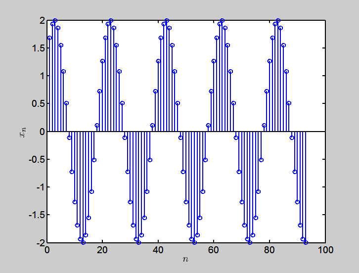
Figure 1
事实上Fig. 1的序列是一个有一定时延的正弦序列(即不是从零开始),我们已经根据规定的fs知道了它的周期和频率,不仿就把它改作在时间轴上(Fig. 2)。
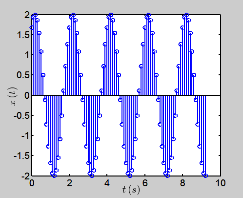
Figure 2
可以看到,该正弦信号的零位在第17和第18个单元之间,即在1.6 s到1.7 s处,以1.6 s计算,该信号可写成![x\left(t\right)=A\sin(\left[2\pi f\left(t-1.6\right)\right]=A\sin(\left(2\pi ft+\delta\right)](https://mlnbqvqmzkw4.i.optimole.com/w:293/h:15/q:mauto/f:best/https://www.andrewsun.net/panta_rhei/wp-content/ql-cache/quicklatex.com-5d8960fccf9a2fdf12300d490089e90a_l3.png "Rendered by QuickLaTeX.com") ,则相位角
,则相位角 ,换成0到2π之间就是
 。若取时移是1.7 s得
 ,所以δ应该在0.9425到1.2566之间。从图中还能读出振幅A = 2,则信号
 。用正弦函数去拟合Fig. 2的序列发现其实最精确的函数描述应该是
 ,见Fig. 3。
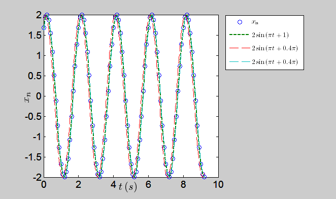
Figure 3
现在我们试着在MATLAB通过Fourier变换来精确地得到xn的幅值和相位,重构一个xn所对应的连续信号。首先构造上述的时域信号:
t = 0:0.1:9.2; % fs = 10 Hz

t = t(:); % convert into column vector

f = 0.5; % f = 0.5 Hz

x = 2 * sin(2 * pi * fi * t + 1)
前面说过对一组N个单元的序列进行Fourier变换之后得到的Xk也是一个N个复数单元的序列。我们看看它长什么样(分开模序列和辐角序列):
Xraw = fft(x);

stem(abs(Xraw),'o'); % Figure 4

stem(angle(Xraw),'o'); % Figure 5
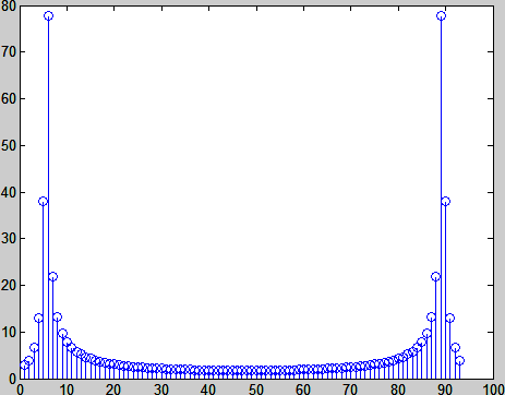
Figure 4
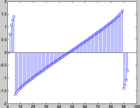
Figure 5
我们从Fig. 4可以看到结果跟我们想像的差很远。主要有以下四个问题:
- 频域谱分成了对称的两半。要取左边一半。但总单元个数为奇数(N = 93),到底是取46个还是47个?
- 若只看一半,频谱出现了单峰是没错(因为我们的信号只有一个频率),但它不是只在一个频率上,而是有一个很宽的分布,似乎我的输入信号的频率是“不纯”的——这并不符合事实
- 幅值不对,信号幅值是2,但频谱的峰高快到80了
- 横轴如何对应到真实的频率轴?
我们一个一个问题地解决。第一个问题,按照fft算法的规律,若N为偶数,则左右分成各N/2的两半即可;若N为奇数,则处于中央的那个单元是左右两半谱共用的。所以,无论取左半还是右半,都取(N+1)/2+1个。综合奇数和偶数的情况,对任意正整数N的取法就是对N/2向上取整。
N = length(x);

Xraw = Xraw(1:ceil(N/2));

stem(abs(Xraw));
第二个问题,之所以频谱的峰有一个很宽的分布,是由于谱泄漏(spectral leakage)现象,简单地说就是我们用来做Fourier变换的信号序列长度并不是恰好整数个周期。只有截取整数个周期来做Fourier变换,才能避免谱泄漏。可是对于一个未知频率的信号,我们本来就是要通过Fourier变换来知道它的频率,又怎么能在此之前就得知信号的周期呢?这种情况下,只能采用另一种方法,那就是把信号的首尾进行某种衰减处理,而这一处理在数学上又要保证不严重影响Fourier变换的结果,称为加窗操作(windowing)。详细的原理不在此详述。作为示范,我们可以利用我们对时域信号的已知信息来解决。已知信号周期T = 2 s,取样频率fs = 10 Hz,到底截取多少个点算一个周期呢?前面计算过了,20个点。干脆我们就只取一个周期得了,试试看:
x_cut = x(1:20); % N = 20

Xraw = fft(x_cut);

Xraw = Xraw(1:10); % N=20, so ceil(N/2) = 10

stem(abs(Xraw)); % Figure 6
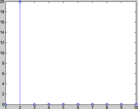
Figure 6
这次,频峰值终于只出现在一个频率上了。而由于用来做Fourier变换的信号N减小到了20个,所以频域信号也就只有20个单元,取左半边就是十个单元。但我们看到,峰值也变了,原来近80,现在是在20。这说明,这个不正确的峰值,是跟N值有关的。这就涉及到第三个问题:峰值怎么校正回来。其实,我们做离散Fourier变换,需要进行归一化。但是怎么归一化,要看离散Fourier变换和反Fourier变换的具体规定,不同的书规定不一样。MATLAB里fft命令是需要用N来归一化的。但如果出来双面的频谱,各边就要用N/2来归一化。所以进行了归一化的的Fourier变换操作应为:
Xraw = 2 * fft(x_cut) / 20;

Xraw = Xraw(1:10);

stem(abs(Xraw));
出来的结果,峰值就会准确落在2(图略)。现在剩下最后一个问题,那就是横轴怎样换成真正的频率?这就要先了解Shannon-Nyquist定理。在此我只把结论说出来:频域信号单元的间格频率是fs/N。因此整个左半边谱的频率范围就是0 Hz ~ fs/2 – fs/N。为了解决奇数偶数问题(即以防fs/2不一定是fs/N的整数倍),最终我们就如下构造相应的频率轴:
freq = 0:fs/20:(ceil(N/2)-1)*fs/N;

freq = freq(:);

stem(freq,abs(Xraw)); % Figure 7
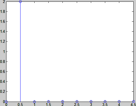
Figure 7
其实,要取整数个周期,不一定要只取一个周期。原时域信号至少有4个周期(见Fig. 1),所以我们可以取满整4个周期来做Fourier变换:
x_cut = x(1:80); % 4 cycles = 80 points

Xraw = 2 * fft(x_cut) / 80; % N = 80

Xraw = Xraw (1:40);

freq = 0:fs/80:fs/2-1/80;

stem(freq,abs(Xraw)); % Figure 8
Figure 8
可见,当我们多取几个周期时,Fourier变换的结果频率“分辨率”更高。因此为了获得尽可能完整地信息,要在保持取整个周期的同时,尽量取最多个周期来进行Fourier变换。我们把相应的辐角谱也作出来:
stem(freq,angle(Xraw); % Figure 9
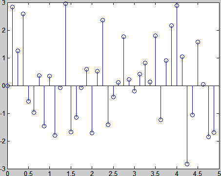
Figure 9
我们发现,跟Fig. 5相比,Fig. 9的辐角谱显得非常杂乱无章。这是由于我们很好的消除了谱泄漏。规律:谱泄漏越严重,辐角谱越有序;谱泄漏避免得越彻底,辐角谱就越杂乱无章。虽然杂乱无章,但是模谱的幅值所在相应频率对应的辐角是应该是正确的。我们看看0.5 Hz处的辐角:
wrapTo2Pi(angle(Xraw(5))) % wrap result within 0 to 2Pi
结果不对,这是由于在MATLAB的fft得到的辐角差了π/2,要加上:
wrapTo2Pi(angle(Xraw(5))+0.5*pi)
这次就对了。
问题是,在实际应用中,我们不可能做一个Fourier变换,就作一次图,用肉眼看出峰值落在哪个频率上。必须事先就知道信号频率f在频域信号中的对应序号,直接就给出模的峰值和相应的辐角。所以,现在的问题是,如何不通过作图就知道,对于一个频率为f,采样频率为fs,N个单元的信号xn,进行了上述的Fourier变换后得到的Xk,第几个单元呢对应着f?这很简单,Fourier变换后的频率间隔是fs/N,因此,第Nf/fs+1个单元就是模的峰值所在频率。本例子中既可验证。
但是,假如信号的频率f在Fourier变换之后的频率轴上的位置,是恰好在频域信号两个单元之间呢?例如,我的信号频率是f=0.51 Hz,fs和N值不变,按照上述算法,要取第5.08个单元,当然不存在这个非整数单元。这就是说,我们要对Nf/fs+1这个公式加一个四舍五入的取整。注意,由于信号频率不同了,“整数个周期”的截取可能会略有不同。以下是具体的运算过程:
f = 0.51

x = 2 * sin(2 * pi * f * t + 1);

N = length(x);

N_per_cycle = fs/f; % average points per cycle

N_cycles = floor(N / N_per_cycle); % maximum number of complete cycles

N_cut = round(N_cycles * N_per_cycle); % number of points for FFT

x_cut = x(1:N_cut);

Xraw = 2 * fft(x_cut) / N_cut;

Xraw = Xraw(1:ceil(N_cut/2));

freq = 0:fs/N_cut:fs/2-fs/N_cut;

abs(Xraw(round(N_cut*f/fs)+1))

wrapTo2Pi(angle(Xraw(round(N_cut*f/fs)+1))+0.5*pi)

freq(round(N_cut*f/fs)+1)
结果离真实值就稍有偏差。这时,如果我们试试把fs提高到1000 Hz。
clear all;

fs = 1000;

t = 0:1/fs:9.2;

t=t(:);

f = 0.51

x = 2 * sin(2 * pi * f * t + 1);

N = length(x);

N_per_cycle = fs/f; % average points per cycle

N_cycles = floor(N / N_per_cycle); % maximum number of complete cycles

N_cut = round(N_cycles * N_per_cycle); % number of points for FFT

x_cut = x(1:N_cut);

Xraw = 2 * fft(x_cut) / N_cut;

Xraw = Xraw(1:ceil(N_cut/2));

freq = 0:fs/N_cut:fs/2-fs/N_cut;

A = abs(Xraw(round(N_cut*f/fs)+1))

delta = wrapTo2Pi(angle(Xraw(round(N_cut*f/fs)+1))+0.5*pi)

frq = freq(round(N_cut*f/fs)+1)
结果就比之前更接近真实值了。这说明,时域信号的采样频率越高,越有利于精确地重构。现在可以看一下重构的效果:
x_rec = A * sin(2*pi*frq*t+delta);

plot(t,x,'bo',t,x_rec,'r-') % Figure 10
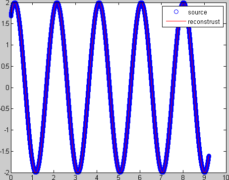
Figure 10
下一篇文章会介绍当原时域信号的频率“不纯”的时候如何通过Fourier变换进行重构。